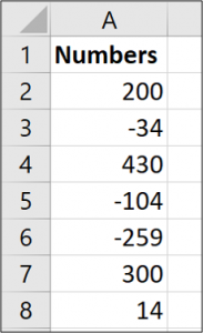
Microsoft Excel displays negative numbers with a leading minus sign by default. It is good practice to make negative numbers easy to identify, and if you’re not content with this default, Excel provides a few different options for formatting negative numbers.

Excel provides a couple of built-in ways to display negative numbers, and you can also set up custom formatting. Let’s dive in.
Change to a Different Built-In Negative Number Option
One thing to note here is that Excel will display different built-in options depending on the region and language settings in your operating system.
For those in the US, Excel provides the following built-in options for displaying negative numbers:
- In black, with a preceding minus sign
- In red
- In parentheses (you can choose red or black)
In the UK and many other European countries, you’ll typically be able to set negative numbers to show in black or red and with or without a minus sign (in both colors) but have no option for parentheses. You can learn more about these regional settings on Microsoft’s website.
No matter where you are, though, you’ll be able to add in additional options by customizing the number format, which we’ll cover in the next section.
To change to a different built-in format, right-click a cell (or range of selected cells) and then click the “Format Cells” command. You can also press Ctrl+1.


